Activity 18: Convolutional Neural Networks

🕑18:47, 1 Dec 2019

Introduction

For this activity [1], I will be using the Keras API with the TensorFlow backend with GPU support to make training faster, to easily monitor loss values and metrics, and quickly tune the network’s hyperparameters to our liking. All experiments were performed on a laptop running on Windows 10, Intel Core i5-7300HQ, 24GB RAM, and an NVIDIA GeForce GTX 1060 with 6GB VRAM.

Dataset

I will be using this dataset [3] for training and this dataset [2] for testing. Both datasets contain thousands of color images of cats and dogs that are roughly equally distributed. The images are not staged so they may contain other objects in the frame other than the intended subject, or even more than one cat/dog. The images are named by the class label followed by its sequence number (e.g., cat.0001.jpg). This makes it easier to pre-process later on.

Input pipeline

We store the image filenames in a dataframe and not the images themselves. This is because due to the number of images, it is unlikely that they will fit in the GPU memory all at once. After a few trials, the optimal batch size was determined to be 128. This means that only 128 images will be in memory at a time. The data flow is as follows:

1. Image is read from persistent storage (such as a hard drive).
2. Image is loaded to RAM and CPU performs pre-processing.
3. Image is copied to GPU memory for training.

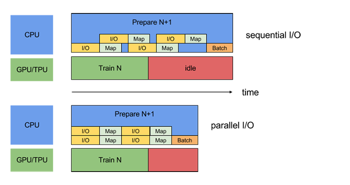
Transfer from RAM to GPU contributes most of the overhead, and usually, the GPU can be trained on the entire dataset much faster than the CPU can preprocess it. In order to optimize the use of resources, we parallelize the CPU and GPU operations such that the CPU prepares the next batch while the network is being trained on the GPU. A visualization of the parallelization as compared to standard serial programming is shown in Fig. 1.

Pre-processing

Upon importing the images from disk, we rescale the image so that its values take up the range . Next, we augment the data by performing random affine transformations such as rotation, shear, flip, zoom, and translation. Finally, all images are reshaped to px. 20% of the training set will be reserved for validation. The parallelization scheme will be handling the batching of the images.

Architecture

Our convolutional network architecture draws ideas from the designs of [4, 5]. The visualization of the network is shown in Fig. 2.

Our input image has a dimension of . The first layer is a 2D convolutional layer with 32 filters and a kernel size of , followed by a ReLU activation, and then by a max pooling layer with a pool size of and a stride of 2. This is succeeded by 3 more layers which repeat the same sequence, but with 64, 128, and 128 convolution filters, respectively. After the last convolutional layer, a dropout layer with a factor of 0.5 is employed. This randomly sets a fraction of the previous layer’s weights to zero---in this case, half of the weights---to prevent overfitting. This is followed by a 512-unit fully-connected layer, activated by ReLU. The output layer is a lone fully-connected unit which is activated by a sigmoid. All layers are initialized with a random Gaussian distribution of zero mean and unit standard deviation, and all biases are initialized to zero. Because our output has only one node but we expect it return a binary value, we select our loss function to be the binary cross entropy, defined as

where is the label, and is the predicted probability of an image of having label for all images [8]. For the optimizer, we use stochastic gradient descent (SGD) with learning rate , momentum , and a decay of . We also use a learning rate scheduler, which reduces the learning rate by a factor of 10 if the validation loss does not improve over 5 epochs. Lastly, we also utilize a checkpointer, which saves a snapshot of the model weights if the validation loss decreases after an epoch. While monitoring the loss and accuracy, we now train the network until the validation loss drops below 0.1 or when the validation loss starts to diverge from the training loss.

Results and Discussion

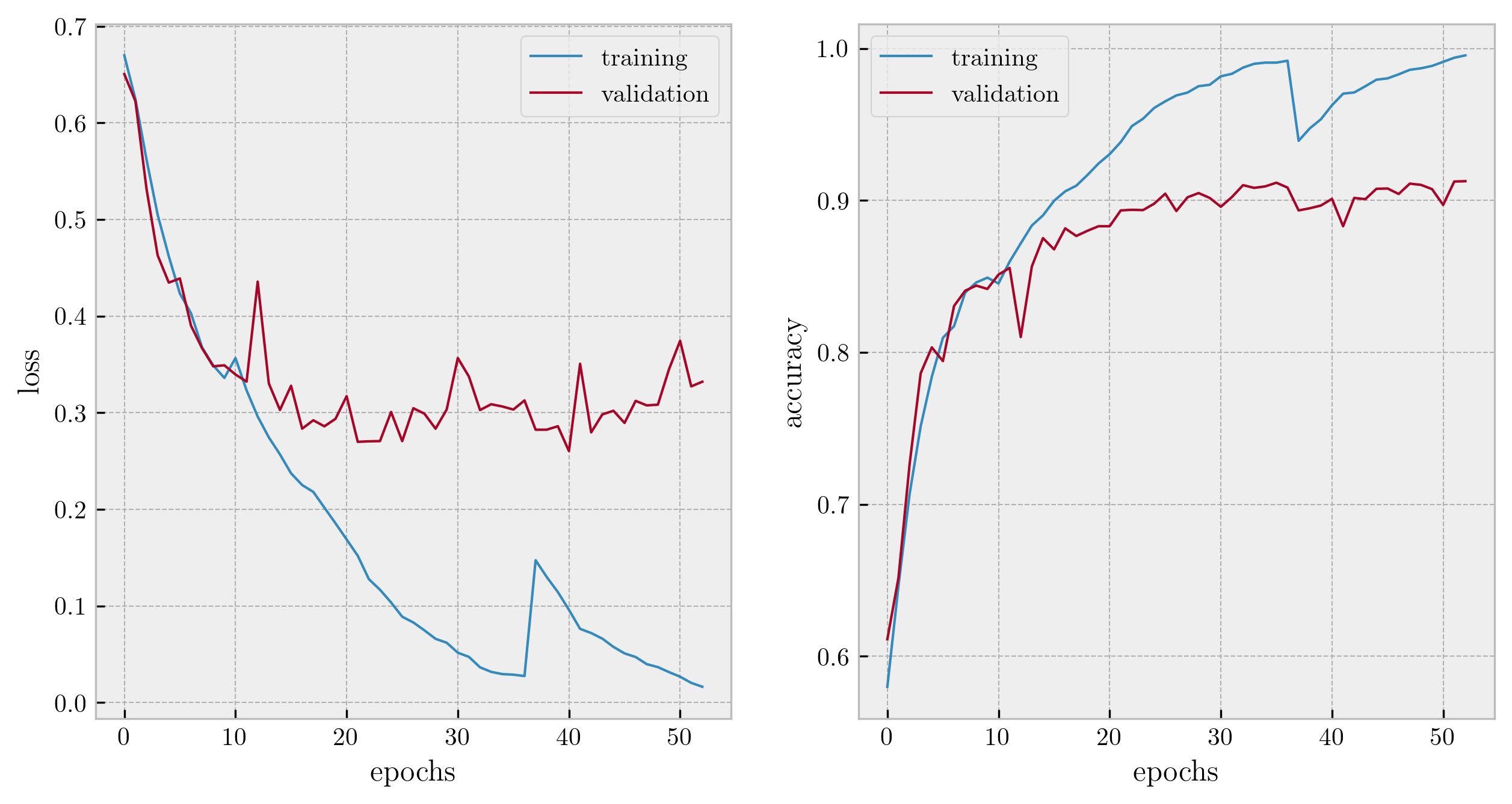
Figure 3 shows the loss and accuracy curves after training the network. At around epoch 20, the validation loss and accuracy start to level out. Training was manually stopped at epoch 53 after observing no further improvement in validation loss. We restored the best weights which were obtained at epoch 40, which had a validation loss and accuracy of 0.26 and 90.10%, respectively. Overall training took around 45 minutes.

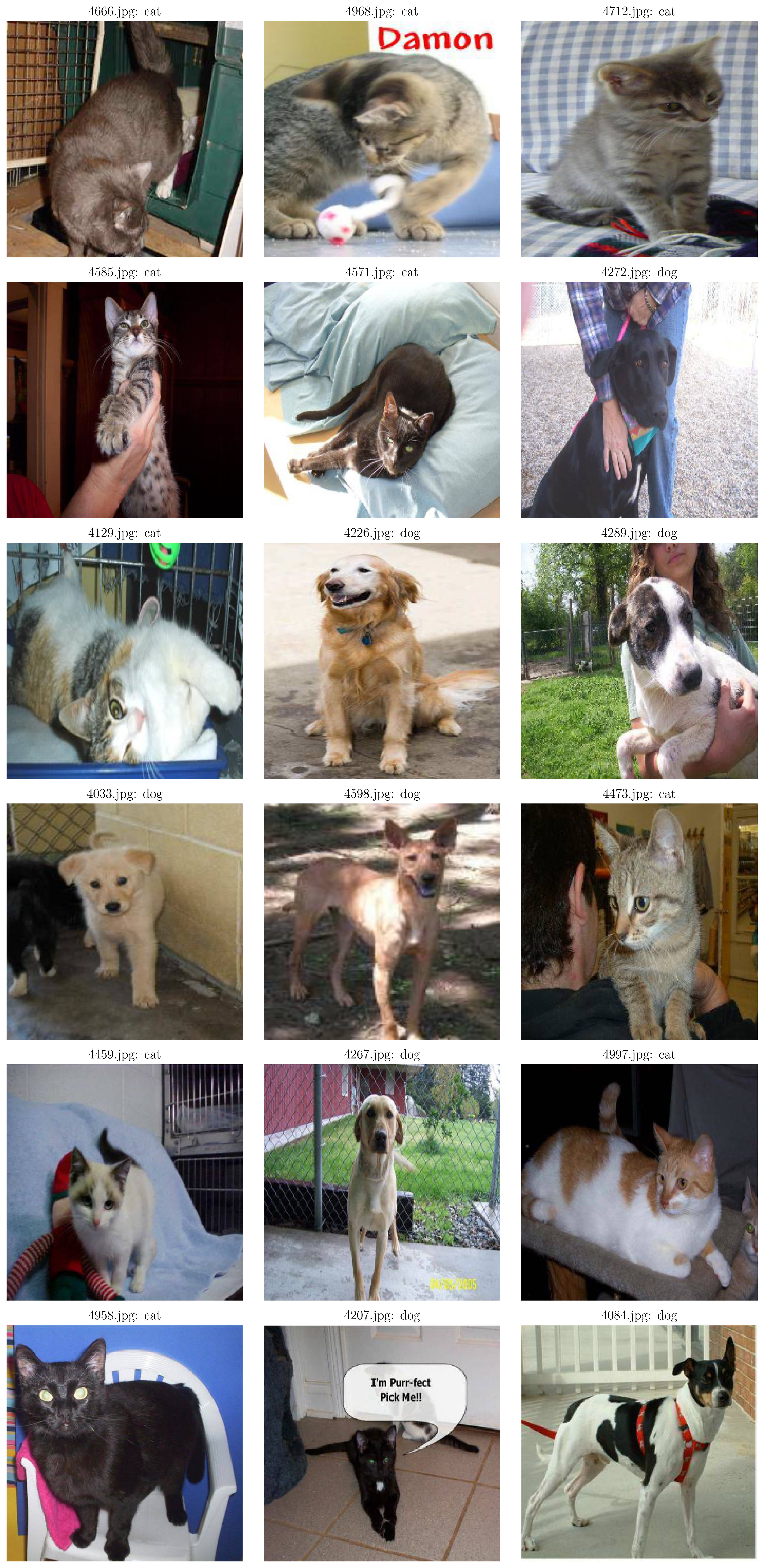
Feeding the test images in the network yields a loss of 0.09 and an excellent 97.03% accuracy. Sample predictions are shown in Fig. 4. Only one out of the 18 predictions is wrong. Upon observation, we can see why the network may have been confused: due to the dark color of the cat.

For increasing the accuracy of the network, one may consider adding another dropout layer after the deep fully-connected layer, playing around with the convolutional layer parameters, and using a deeper network.

References

1. M. N. Soriano, A18 - Convolutional neural networks (2019).

2. Kaggle, Cats and dogs dataset to train a DL model (2017).

3. Kaggle, Dogs vs cats (2015).

4. A. Krizhevsky, I. Sutskever, and G.E. Hinton, ImageNet classification with deep convolutional neural networks. Advances in Neural Information Processing Systems 25 1097-1105 (2012).

5. L. Strika, Convolutional neural networks: A Python tutorial using TensorFlow and Keras (2019).

6. A. Agarwal, Building efficient data pipelines using TensorFlow (2019).

7. A. LeNail, Publication-ready neural network architecture schematics, Journal of Open Source Software 4(33) 747 (2019).

8. D. Godoy, Understanding binary cross-entropy/log loss: a visual explanation (2018).

Keywords